

Introduction to CMS OpenPayments Data Analysis using Machine Learning
In the previous blog we discussed the fundamental concept of what Machine Learning is and how it can be applied in the modern world of Pharmaceuticals and Healthcare, further to this we explored CMS Open Payments, the federal program that collects information about the payments drug and device companies make to their potential clients.
Now that we’ve had our brief introduction into the world of Machine Learning and Healthcare related use cases, we can start to factor in the types of ML Algorithms that we can apply to these Pharma specific datasets. Don’t worry though, it’s easy to become overwhelmed by the vast amount of ML models and their associated metrics, so let’s start from the foundations and build up.
To this end we will be exploring a simplistic and well-known statistical regression algorithm known as Linear Regression.
The Machine Learning Model
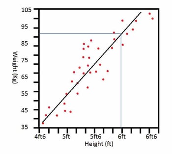
So to get the ball rolling in this regard, what is Regression? Regression is a method representing the correlation between the features of your data and an observed, continuous-valued response. In Layman’s terms, it is essentially the relationship between an input value and an output value. For example, if you were asked to approximate the weight of an individual based solely on features of their appearance, you’re first instinct could be to judge how tall the person is, as you automatically assume that as someone’s height increases, their weight would also increase proportionally. This is Regression in its rudimentary form [1]. This example can be visualised as follows:

Now let’s get a little bit more specific by asking, what is Linear Regression?As this is the model I will be experimenting with throughout the later duration of these blogs. Linear Regression is a very simple approach to supervised learning. Though it may seem somewhat dull compared to some of the more modern algorithms, it is still a useful and widely used statistical learning method. Linear Regression is used to predict a quantitative response y from the predictor variable x, but this is made with the assumption that there’s already a linear relationship between x and y.
There are two main types of Linear Regression:
- Simple Linear Regression: Uses one x input predictor value;
- Multiple Linear Regression: Uses more than one x input predictor values.
For the purpose of this exercise, we will be sticking with Simple Linear Regression, but I will also be exploring the usage of Multiple Linear Regression in the following blog.
When working with a data set in the hopes of applying an ML model, it’s normally advised to become thoroughly familiar with the data, what it means, and to establish whether there is any form of correlation between the data’s various features. In order to represent this correlation, we employ the use of the least squares line of best fit, otherwise known as the regression line. This regression line is a plot of the expected output value yfor each discrete input value x, with our aim to position the line so as to minimize the sum of all the squared distances from the line to the actual data points [2]. The following video posted by PatrickJMT helps to explain this concept:
The graph pictured above is an image of Simple Linear Regression in relation to the previously stated example about approximating weight judging by an individual’s height. Now let’s jump into the basic theories behind Linear Regression, this will help with our understanding of how to apply it through Machine Learning to any particular dataset.
Mathematically, we can write a linear relationship as:
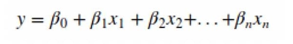
where,
- y is the output response
- β values are called the Model Coefficients. Model coefficients refer to how many standard deviations a dependent variable will change, per standard deviation increase in the predictor variable[3].
- β0 is the intercept. The intercept is the mean value of Y at the chosen value of X.
- β1 is the coefficient for x1 (the first feature).
- βn is the coefficient for xn (the nth feature)[4].
The following video posted by Arduino Startups helps to explain the theory of Linear Regression with regards to Machine Learning:
Previous Applications of Regression in the Pharmaceutical Industry
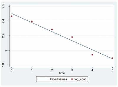
In 2011, the University of Melbourne conducted an experiment into applying a Regression ML algorithm to a pharmacokinetic specific dataset to establish a relationship between the concentrations of drugs present within the body and how this is affected over time due to the rate of absorption. More details on this project can be found in the attached link below:
http://www.wwarn.org/sites/default/files/CompartmentalModelling.pdf
In this example, there are multiple methods of model estimation included to help improve the accuracy such as Ordinary Least Squares (OLS) and Weight Least Squares (WLS). As a result they were able to determine a linear relationship between the drug concentrations with respect to time, this is visually represented below:
Conclusion
Now that we have learned about the basic theory behind Regression algorithms, we can start to look into how to apply these models to a healthcare related dataset and analyse the results that are generated. In the next blog I will be dissecting the code that performs this task, piece by piece, to demonstrate how to effectively apply an ML model to a KDB+ table.
About the Author
Jonathan is a graduate of Software & Electronic Systems Engineering from Queen’s University Belfast who recently joined the technical team at RxDataScience using KDB+ as a go-getting and determined software engineer and data-scientist. From working in such a technical environment alongside RxDataScience he has gained an appreciation for all things machine learning and aspires to learn to a great deal in this ever growing field of industry in the hopes of helping revolutionize the healthcare industry with this game changing new technology.
References
[1] https://www.coursera.org/learn/ml-regression
[2] https://www.statpac.com/statistics-calculator/correlation-regression.htm
[3] https://en.wikipedia.org/wiki/Standardized_coefficient
[4] https://medium.com/simple-ai/linear-regression-intro-to-machine-learning-6-6e320dbdaf06
