

Using Support Vector Machines
This is part 2 in a 2 part series about Pharma Machine Learning and Healthcare, using breast cancer diagnosis as an example application.
Recap: The Problem
My previous blog post discussed the uses of Machine Learning (ML) in Healthcare and introduced the breast cancer biopsy classification problem. We would like to create a classification model that can identify digitized microscope slides as cancerous or non-cancerous based on cell descriptors such as radius, texture and symmetry. This post will introduce Support Vector Machines (SVMs), the algorithm that will be used for biopsy classification.
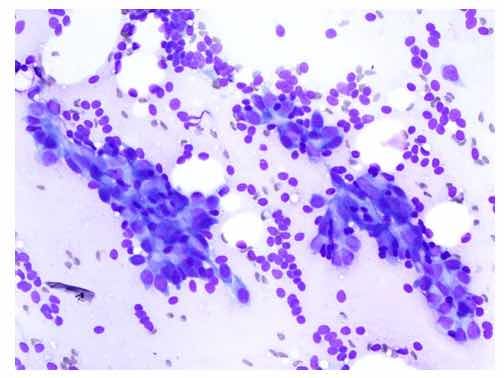
Figure 1: Sample from breast mass fine needle aspiration biopsy.
Support Vector Machines in Healthcare
SVM classifiers (SVCs) are a type of supervised learning model commonly used for high dimensional binary classification problems. This means that SVM classifiers are effective at dividing data with many features into two groups.
In healthcare, SVCs have been investigated as a method to automate the collection and extraction of genomic information from large quantities of published articles on biological databases. They have also be researched as a method to detect cases of diabetes in the U.S. population based on age, gender, health factors, family history and more. Adaptations of the classic SVM can be used for multiclass problems, for instance to predict which of four classes of heart failure a patient falls into based on socioeconomic and health assessment results.
What does an SVM do?
For a set of data in dimensional space, where is the number of features, a binary SVC classifies data by identifying a dimensional hyperplane that separates the two groups.
In the example below, data has 2 features, thus the SVM hyperplane is a line. However, we see that there are many possible lines that can divide the data classes. So how is the best separating hyperplane determined?
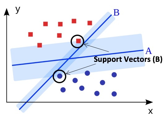
Maximum Margin
To optimize the hyperplane, we use a metric known as maximal margin. This is the distance between the hyperplane and the data points that lie closest to the hyperplane on either side, points known as support vectors. As we see below, planes A and B both separate the red and blue classes, but plane A maximizes the distance between support vectors and the plane and is therefore the optimal solution. Through maximum margin optimization we are minimizing the risk of making incorrect decisions when the model is applied to new data.
The C Parameter
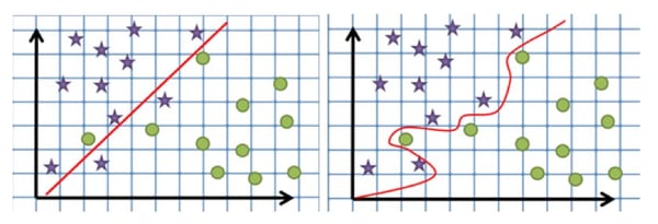
In some cases, building a model that classifies all training points correctly can lead to a poor classifier that is overly specific to the data used for building the model. In such cases, allowing outliers to be misqualified during training will lead to a better overall model. In the left image below, a simpler separating model is created by allowing some data points to be misqualified. The right image shows a hyperplane that has been tightly fitted to the data and is thus overcomplicated and less likely to correctly predict classes for new data.
To address this, a ‘soft-margin’ is used, allowing some points to be ignored or placed on the wrong side of the hyperplane. The C parameter, or soft margin cost function, controls the influences of each individual support vector, thus controlling the trade-off between properly classifying all points during building the model, and a smooth decision boundary which will generalize well for future predictions.
Kernel Trick
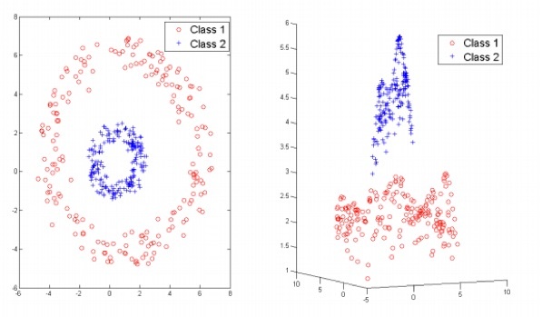
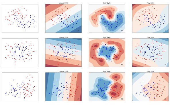
So far we have illustrated principles of SVMs using linearly separable data; however this will not always be the case when looking at real datasets and a linear SVM will fail to identify an effective separating plane. This is where the kernel trick comes in. A kernel is a function that maps data to a higher dimension, where it can linearly divided.
The differences between three common kernel functions – linear, radial basis function (RBF) and polynomial – are illustrated bellow, though other kernel options exist and it is also possible to create your own.
The Gamma Parameter
Similar to the C parameter, the gamma parameter, or kernel coefficient, dictates the level of complexity in the kernel fitting.
Putting it all together
Grid Search and Cross Validation
The C parameter, kernel function and gamma parameter can be tuned to improve our model and identify the optimal hyperplane to separate data into cancer and non-cancerous classes.
To do this we will employ scikit-learn’s Grid Search method, which constructs grid of all potential parameters combinations and a model with each combination. A section of training data is set aside for evaluation each of model and is used to generate a cross validation score. A higher cross validation score is indicative of a better combination of parameters.
Scoring the model
There are a number of scoring functions that can be used to evaluate model. Accuracy, perhaps the most obvious metric, quantifies the number of correctly identified data points over the total number of data points. However the number of correct points is not always the best metric to evaluate a model. For a cancer diagnosis model, the worst case scenario is that a patient is incorrectly told that they do not have cancer and do not receive required treatment. Thus we will want to use scoring metrics which allow the model to be tuned to minimize false negatives.
In Summary
Support Vector Machines divides classes by identifying a separating hyperplane in a dimensional space one less than the number of features of the data. An SVM model will be used classify breast cancer biopsy slides as cancerous or non-cancerous using 30 different nuclei features. Penalty (C), kernel type, gamma and other parameters will be tuned using grid search to identify the optimal model.
