

Introduction
According to the Centers for Medicare and Medicaid Services, the National Health Expenditure in the United States reached 3.2trillionin2015,whichmakesit9,990 per person per year [1]. Such huge expenditures on healthcare may not lead to affordable healthcare to patients [2]. Therefore, it is crucial to predict the likely future patient-related expenditures to help patients better manage their huge healthcare costs. Predicting the healthcare expenditure may also be useful for various other stakeholders that include drug manufacturers, health insurers, pharmacies, and hospitals. Here, developing accurate healthcare expenditure models may help patients to choose appropriate insurance plans and may help healthcare delivery systems in better business planning [3].
Healthcare datasets mostly contain hundreds of variables such as demographic information, health-plan related information, medicine purchase information, diagnoses, and procedure codes [4]. Therefore, choosing the right set of healthcare variables and predicting the healthcare expenditures accurately is a challenging problem. Prior researchers have performed healthcare expenditure predictions by developing regression [5]–[6][7] and classification techniques [8], [9]. Most of the prior studies have used classical data mining approaches such as decision tree [10], random forest regression [11], multiple linear regression [11], clustering [8], bagging [10], and gradient boosting [10] for healthcare expenditure predictions. Here, some of the prior studies have relied upon the specific patient population (which may lead to non-generic results), used uncorrelated healthcare variables, or variable with very limited predictive accuracy [12]–[13][14].Some of the recent studies in the healthcare domain have addressed prediction problems as time-series forecasting problems [15]–[16][17][18]. Here, researchers have shown that statistical time-series methods like autoregressive integrated moving average (ARIMA) models do not work for predicting healthcare data [18]. A likely reason is the pre-assumption of linearity in the underlying time-series by these methods [19]. Since time-series variables may depict non-stationary and non-linear behavior, neural networks may be considered as a preferred choice for time-series predictions in practical scenarios [19]. That is because neural networks, with different assumptions on activation functions and hidden layers, may account for the non-stationary and non-linear behavior in time-series variables [19]. Recently, certain neural network architectures such as multilayer perceptron (MLP), long short-term memory (LSTM), and convolutional neural network (CNN) have been proposed for predicting time-series involving healthcare expenditures with some success [15]–[16][17][18].
Furthermore, a class of generative neural network models called generative adversarial network (GAN) has been proposed in the literature [20]. GANs are trained as a min-max game, where a discriminative neural network learns to distinguish whether the supplied data instance is real or fake, and a generative neural network learns to confuse the discriminator by generating high-quality fake data [20], [21]. One seeks the convergence of the combined generator-discriminator model by minimizing a chosen loss function [21].
Mostly, binary cross-entropy (also called as log loss) has been used as the loss function to train GAN models [21]. However, the binary cross-entropy loss function may not provide a sufficient gradient for the generator model to learn as quickly as the discriminator model [20]. Therefore, alternate loss functions like the least-square loss [22] and the Wasserstein loss [23] have been proposed in the literature. Recent research has shown that the least-square loss may lead to the problem of vanishing gradients when updating the generator model [22] and the Wasserstein loss (calculated as the distance between two probability distributions in terms of the cost of turning one distribution into another) shows better properties of convergence compared to the least-square loss [23].
By relying upon different loss functions for the generator and discriminator models, GANs have been successfully developed for a wide range of applications such as semantic segmentation [24], image inpainting [25], stock market prediction [26], and video prediction [27], [28]. However, to the best of authors’ knowledge, the development of GANs and its variants for performing time-series prediction of future healthcare expenditures has not yet been explored in literature. We overcome this literature gap in this research by proposing a novel GAN architecture called variance-based GAN (or V-GAN) for the time-series predictions of healthcare expenditures.
Different from prior studies, we introduce a variance term in the V-GAN’s loss function that explicitly minimizes the difference in the variance between patient data and model data during model training. Thus, in the new V-GAN model, we train the generator network using a different and novel combination of loss functions, which includes root mean square error (RMSE) loss, binary cross-entropy loss, variance loss, and their combinations. For the discriminator network in the new V-GAN model, we experiment with binary cross-entropy loss function, Wasserstein distance loss function [23], and a novel combination of both these loss functions.
For comparing the performance of the V-GAN architecture, we use the following machine learning methods: an ordinary least square linear regression (LR) model [29], a gradient boosting regression (GBR) model [29], an MLP model [18], and an LSTM model [15]. Since the V-GAN model can learn the approximate distributions in training data, we expect the V-GAN model to be able to generate accurate time-series predictions of the healthcare expenditures better than other existing models like GANs, regression models, MLPs, and LSTMs.
In what follows, we first provide a brief review of related work involving healthcare expenditure prediction and GAN models. Then, we explain the data used in this research for model development. Next, we explain the methodology of the new V-GAN model, different GAN variants, and the LR, GBR, MLP, and LSTM models. Furthermore, we present our experimental results, and we conclude the paper by discussing the implications of this research and its possible extensions.
Related Work
A. Healthcare Expenditure Prediction Methods
Based on prior research, two categories of approaches have been proposed to predict healthcare expenditures: regression models and classification algorithms [5], [8]. The first category involves using classical regression approaches such as ordinary least square (OLS) linear regression to estimate total annual health expenditure of patients in insurance claims data [5], [6], [30], [31]. For example, Moran et al. compared generalized linear models and OLS to predict individual patient expenditures in intensive care units [30]. These researchers obtained optimal overall performance from both these models. Marquardt et al. used linear regression and regression trees to develop a data-mining framework for scalable prediction of healthcare expenditures [31]. In recent years, researchers have developed neural network architectures such as MLP, LSTM, and CNN models for predicting patients’ expenditure data [15]–[16][17][18]. Researchers have also compared the neural architectures with statistical time-series methods (e.g., ARIMA model) and found that the neural network models perform better compared to statistical methods for predicting healthcare expenditures [15], [18].
The second category involves the use of classification algorithms, where patients are classified into different expenditure buckets/classes [8], [32], [33]. For example, Bertsimas et al. used classification trees and clustering algorithms to classify patients into five different expenditure classes by using patients’ expenditures and clinical information [8]. Lahiri and Agarwal performed expenditure predictions as a binary classification task to predict whether beneficiaries’ inpatient claim amounts increased or not between 2008 and 2009 [32]. These researchers achieved good performance by using an ensemble of six different classification approaches, which included conditional inference tree, logistic regression, gradient boosting, neural networks, support vector machines, and naïve Bayes. Similarly, Guo et al. performed a predictive modeling approach to predict patients’ transitions from one expenditure bucket to another expenditure bucket [33]. Beyond the classical approaches described above, generative adversarial networks (i.e., networks that use generative and discriminative models in a min-max game) could be developed for predicting healthcare expenditures.
B. Generative Adversarial Networks
Generative adversarial networks (GANs) rely upon two neural networks (a generator G and a discriminator D) that are trained simultaneously in an adversarial manner [20]. The generator model generates the synthetic or fake samples (that can pass for real data) by estimating the data distribution, and the discriminator model estimates the probability that a sample came from the training data or the generator model. Aim of G’s training process is to maximize the probability of D making a mistake. Both G and D are trained against a static adversary. When G is trained, D’s values are kept constant and vice-versa [20], [23].
Goodfellow et al. used MLP models for training G and D [20]. However, recently, researchers have implemented G and D using an LSTM model [34] and a CNN model [35], respectively, for a number of applications [26], [36], [37]. For example, Nie et al.used adversarial training to train a convolutional network for generating computer tomography images (CT) given medical resonance (MR) images [36]. The experimental results showed that the proposed method was accurate and robust for predicting CT images from MR images and could be used for medical image synthesis tasks. Researchers have also proposed a speech enhancement generative adversarial network (SEGAN) architecture for speech enhancement using GAN frameworks [37]. SEGAN architecture worked end-to-end by learning from different speakers and noise conditions such that model parameters were shared across these speakers and different noise conditions. Experimental results showed that the SEGAN model was generalizable and required no explicit assumption about the raw data. Zhou et al. have proposed a GAN framework to forecast high-frequency stock market data [26]. The authors trained a GAN model using data provided by a trading software, where G was trained using an LSTM, and D was trained using a CNN model. Experimental results showed that the proposed framework could effectively improve the stock price’s direction prediction accuracy and reduce forecast errors [26].
Although the literature has proposed models for healthcare expenditure prediction, to the best of authors’ knowledge, this paper is the first to adopt a GAN approach for predicting patients’ expenditures on medications. In this paper, we propose a new V-GAN model and compare it with other GAN variants, regression-based models such as LR, GBR, and neural network models such as MLP and LSTM to predict patient-related expenditures on a medication.
Method
A. Data
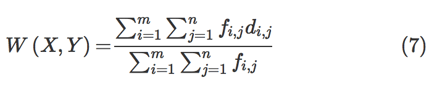
A popular pain medication’s purchase data from the Truven MarketScan dataset [4] was used for model evaluations in this paper. The selected pain medication was among the top-ten most prescribed pain medications in the US in 2015 [38].1 The dataset (uploaded on the IEEE data port, DOI: 10.21227/k0mm-jb74) ranged between 2nd January 2011 and 15th April 2015 (1565 days). The dataset between 2nd January 2011 and 30th July 2014 (1306 days) was used for model training, and the dataset between 31st July 2014 and 15th April 2015 (259 days) was used for model testing. On average, each day, about 1,428 patients refilled the selected medication. The dataset was a multivariate time-series dataset consisting of 21 attributes, which included the daily average expenditures by patients for purchasing the medication. The 20 attributes provided information regarding the number of patients of a particular gender (male, female), the number of patients in a particular age group (0-17, 18-34, 35-44, 45-54, and 55-65), the number of patients from a US region (south, northeast, north-central, west, and unknown), the number of people in a certain health-plan (two types of health plans), and the number of patients belonging to different diagnoses and procedure codes (six ICD-9 codes) who consumed medicine on a particular day. These 6 ICD-9 codes were selected using the frequent pattern mining Apriori algorithm [39], and the selection procedure is reported in a separate publication [40]. The 21st attribute was the average expenditure per patient for the medicine on day t , and it was defined as per the following equation:
Next, the daily average medicine expenditure was used to compute the weekly average expenditure. For computing the weekly average medicine expenditure, the daily average medicine expenditure was summed over a 7-day block. This resulted in the weekly average expenditure across 186 blocks of training data (1306 days were used in training), and 37 blocks of test data (259 days were used in testing). Fig. 1 shows the weekly average expenditure (in USD per patient) of the 21st attribute over weekly blocks. The weekly average expenditure (per block) was used to evaluate different models. We used the Root Mean Square Error (RMSE) to evaluate the performance of different models. The RMSE was computed between model predictions and real data at the block-level.
The weekly average expenditure (in USD per patient) over blocks. Each block is a 7-day period.
B. Prediction Model
In this research, we developed a V-GAN model for generating time-series predictions about patient-related expenditures. Since long short-term memory (LSTM) models are widely used for time-series prediction problems [15], we chose LSTM as a generator model (G) to generate predictions based on an input noise. The task of a discriminator model (D) is to estimate the probability of whether a sequence comes from real samples or the generated (fake) samples. The D works as a classifier that has to correctly classify the input samples as real or fake. Since convolutional neural network (CNN) models are mostly used for classification-based tasks [43], [44], they have been used as the D. As the CNN model is used as the D in prior literature for implementing GAN [26], we chose a CNN model as one of the D models in this research. Additionally, we also implemented the V-GAN model with an MLP as the D (since an MLP was used as the D by Goodfellow et al. [20] in the original GAN paper). It is important to note that the architectures of G and D could be adjusted based on the specific application and could be fine-tuned based on underlying time-series to enhance predictive performance.
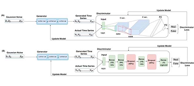
For developing the V-GAN architecture (shown in Fig. 2(A)) for time-series prediction, the G (an LSTM) received an input dimension of 1×21 from the Gaussian distribution. For training the G, we varied the number of hidden layers (1, 2, and 3), the number of neurons (8, 16, 32, and 64), activation function (ReLU, tanh, sigmoid, and leaky ReLU), and the dropout rate for each hidden layer (20% and 30%). For training the D, we used 1×21 dimension input from the real samples and 1×21 dimension input generated by the G. As shown in Fig. 2(A), we passed the Gaussian noise represented as Z1, Z2,… , Z21, an input dimension of 1×21 in a batch size of 64 to the G, which made 64×1×21 as the input shape of the G. In the fully trained V-GAN model, the G contained one LSTM hidden layer with 32 neurons and a ReLU activation function [45]. It was followed by a dropout layer with a 20% dropout rate, and finally, a dense layer with neurons equal to the input data dimension, i.e., 21. Thus, the G’s output shape was the same as the input shape, i.e., 1×21 . From the G, we obtained the fake time-series of 21 dimensions represented as y^1,y^2,…,y^21 in Fig. 2(A). Next, the D was trained using both the real data and fake (generated) data.
The V-GAN architecture. (A) The Generator model (G) was developed using an LSTM model, and the Discriminator model (D) was developed using a CNN model. The “Conv.” and “FC” are abbreviations for the convolutional layers and a fully connected layer, respectively. (B) The Generator model (G) was developed using an LSTM model, and the Discriminator model (D) was developed using an MLP model.
When CNN was used as the D, we varied the same range of hyper-parameters as the G along with the number of filters (32, 64, or 128) and different kernel sizes. The D received the generated time-series represented as y^1,y^2,…,y^21 and actual time-series represented as Y1, Y2,… , Y21 in a batch size of 64. In the CNN-based D, the architecture was composed of two 2D convolution layers followed by two fully connected (FC) layers. The first convolution layer contained 32 filters of 32×4 kernel size, singe-stride, and the leaky ReLU (LReLU) activation function with slope =0.01 [45]. Second, convolution layer contained 64 filters, 64×4 kernel size, single-stride, and LReLU activation function with slope = 0.01. Padding was done in both the convolution layers to keep the input and output shapes the same. Fig. 3 shows the complete convolution operation (inside the D model) in detail. As shown in Fig. 3(A), the first 2D convolution layer received input of shape 64×1×21×1 , where 64 represented the batch size, 1 represented the height, 21 represented the width, and 1 represented the number of channels. For the 2D convolution operation, 32 filters with a kernel size of 32×4 and a single stride were applied. In order to match the kernel size (height and width), 31 rows and 3 columns were padded, making the new data height = 32, and data width = 24. The output shape of the first convolution layer was 64×1×21×32 (batch size × height ×width × channels). The difference in the input and output shapes was just in the number of channels, as 32 filters were applied in the convolution operation. Fig. 3(B) shows the second convolution layer operation using 64 filters with a kernel size of 64×4 and a single stride. Similarly, to match the kernel size, 63 rows (assuming 32 above the actual data row and 31 below the actual data row) and 3 columns (assuming 1 column in front and 2 columns at the end) were padded to the data. The padding made the new data height = 64 and data width = 24. The output shape of the second convolution layer was 64×1×21×64 (batch size × height × width × channels). The output of the second convolution layer was flattened (1×21×64=1344 ; output shape of flatten layer =64×1344 ) and passed to the first FC layer which contained 64 neurons and the LReLU activation function with slope = 0.01 (the output shape of first FC layer =64×64 ). The first FC layer was followed by a second FC layer with 1 neuron and a sigmoid activation function (output shape of second FC layer =64×1 ).
The convolution operation in the discriminator model. (A) Shows the input and output of the first 2D convolution layer, and (B) shows the input and output of the second 2D convolution layer.
As stated above, we also developed the V-GAN architecture with an MLP as the D. Fig. 2(B) shows the architecture where V-GAN was implemented with LSTM as the G and MLP as the D. For developing this architecture, we kept the G (LSTM) architecture the same as described above in Fig. 2(A). For developing the MLP-based D architecture, we varied the number of hidden layers (1, 2, 3, and 4), the number of neurons (8, 16, 32, and 64), activation function (ReLU, tanh, sigmoid, and leaky ReLU), and the dropout rate for each hidden layer (20%, 30%, and 40%). As shown in Fig. 2(B), the final D was trained with one hidden layer containing 32 neurons and the ReLU activation function. The second hidden layer contained 64 neurons and the ReLU activation function, followed by a dropout layer with a 40% dropout rate. The third hidden layer contained 16 neurons and the ReLU activation function, followed by a dropout layer with a 40% dropout rate. At last, the output layer contained 1 neuron with a sigmoid activation function.
The D’s output indicated whether the input sample was real (supplied from the actual time-series) or fake (supplied from the generated time-series). The G aimed to confuse the D such that it could not guess correctly and would give a 50% probability of a sample being fake. Therefore, in the result section, we have also shown the percentage of real-like samples (i.e., fake samples reported as real) reported by the D. The complete model was trained for 20,000 epochs with 64 batch size and using the stochastic gradient descent (SGD) optimizer [46], initialized with 0.01 learning rate, and 0.9 momentum. Additionally, the GAN-based prediction models generated all the 21 attributes on the daily-level. However, the performance of all models was compared based on the predictions obtained for the average daily expenditure, i.e., the 21st attribute.
C. Different Loss Functions
In this section, different loss functions used across different models, including the V-GAN model, are discussed.
1) Adversarial Loss (LA )
In the original GAN paper [20], the adversarial loss was used to evaluate the distance between two probability distributions. Adversarial loss is derived from the cross-entropy between the real and generated distributions, defined as LA in (2) below:
2) Variance Loss (LB )
Variance is used to measure the deviation from the mean. The variance loss (LB ) minimized explicitly the squared difference of the variances between the generated data and the actual data as defined in the following equation:
3) Forecast Error Loss (LC )
In order to improve the forecasting performance of time-series models, researchers have proposed the forecast error loss or the RMSE loss (LC ) [26]. The idea behind using forecast error loss function is to bring predicted data closer to the actual data. Forecast error is defined as per the following equation:
4) Wasserstein Distance Loss (LW )
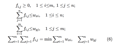
Wasserstein distance is a loss function that measures the distance between the data distribution observed in the training samples and the distribution observed in the generated samples [23]. Arjovsky et al. have shown that training the generator may seek a minimization of the distance between the distribution of the data observed in the training dataset and the distribution observed in generated samples for better convergence and stable training [23]. The Wasserstein distance loss function is a measure of the distance between two probability distributions over a region D. The Wasserstein distance between two distributions X and Y is defined as the minimum amounts of work done to match X and Y, normalized by the total weight of the lighter distribution. Assume that the distribution X has m clusters with
X=(x1,wx1),(x2,wx2),…,(xm,wxm) , where xi is the cluster representative and wxi is the weight of the cluster. Similarly, another distribution
Y=(y1,wy1),(y2,wy2),…,(yn,wyn) has n clusters. Let
D=[dij] be the ground distance between clusters xi and yj . The objective is to find a flow
F=[fi,j] , where fi,j is the flow between xi and yj , which minimizes the overall work as per the following equation:
D. Different GAN Models
In this research, we developed GAN-based time-series prediction models using novel combinations of above-defined loss functions. Table 1 shows the generator and discriminator models’ loss functions across different GAN models (including the new V-GAN model).

Adversarial GAN: We trained Adversarial GAN (A-GAN) using the adversarial loss function (LA ) for both the G and the D (as shown in Table 1). The adversarial learning helps the G to confuse the D, and it helps the D to classify the input samples as real or fake [20]. Both the G and the D update their cost independently as updating the gradient of both models concurrently cannot guarantee convergence [47].
Variance GAN: The Variance GAN (V-GAN) was developed using a novel combination of LA and variance loss function (LB ), i.e., LA+LB , to train the G. The D in V-GAN model was trained using LA loss function. The reason for trying a combination of LA and LB loss functions was that minimizing adversarial loss alone may not guarantee satisfactory predictions. With just adversarial loss, the G could generate samples to confuse the D; however, those samples may not be close to the actual data. To ensure that the G produced samples that confused the D and the generated samples were close to the actual data, we trained the G using the LB loss function in addition to the LA loss function. The LB specifically minimized the difference in variance between generated and actual data. By developing V-GAN, we ensured that the model reduced the adversarial loss, and the LB part of the loss function in the G ensured that the generated sample means did not deviate much from the actual data means.
Forecast Error GAN: The Forecast Error GAN (FE-GAN) architecture was developed using a novel combination of LA and forecast error (LC ) loss function, i.e., LA+LCfor training the G and LA was used to train the D. The reason for taking this combination was prior work in the time-series domain, where researchers used the forecast error loss function (LC ) [26]. The FE-GAN ensured that the G reduces the adversarial loss as well as the forecast error while generating the fake samples.
Variance and Forecast Error GAN: The Variance and Forecast Error GAN (VFE-GAN) was developed using a novel combination of LA , LB , and LC loss functions (LA+LB+LC ) and the D was trained with LA loss function (as shown in Table 1). By developing the VFE-GAN, we aimed at reducing the variance loss and forecast error along with the adversarial loss while generating the samples from G to confuse the D with realistic samples.
Variance and Wasserstein Distance-1 GAN: The Variance and Wasserstein Distance-1 GAN (VW1-GAN) was developed using a combination of LA and LB loss functions (LA+LB ) to train the G. The D was trained using the Wasserstein distance loss function (LW ) (as shown in Table 1). The reason behind using a combination of LA and LB loss functions for the G was to investigate whether the V-GAN improved its performance by using a different loss function with convergence properties in the D [23]. The use of LW in the D is also motivated from literature, where it may become challenging to obtain Nash equilibrium in a non-cooperative game when adversarial loss (LA) is used in the D [47].
Variance and Wasserstein Distance-2 GAN: Building upon VW1-GAN, we also developed a Variance and Wasserstein Distance-2 GAN (VW2-GAN), where the G was trained using a combination of LA and LB loss functions (LA+LB ) and the D was trained using a combination of LA and LW loss functions (LA+LW ). The reasoning to use VW2-GAN was to explore improvements in the V-GAN by using a combination of LAand LW loss functions. Thus, the minimization of the adversarial loss and Wasserstein distance together in the D may help the G in return to produce better predictions.
Different Models for Comparison
To evaluate the performance of the proposed V-GAN model and other GAN-based prediction model variants, we developed an LR model [8], [29], a GBR model [29], an MLP model [18], and an LSTM model [15], [18] (see Table 2). All the developed models in Table 2 were evaluated in their ability to perform time-series predictions on the medicine expenditures’ data. As shown in Table 2, based upon prior literature [29], we trained the LR and GBR models using the least square loss function. Also as shown in Table 2, the MLP and LSTM models were trained three times using the different combinations of loss functions: variance loss function (LB ), root mean square error loss function (RMSE; LC), and a combination of LB and LC loss functions (LB+LC ), separately. The idea behind using these loss functions for the MLP and LSTM models were to evaluate the variance minimization during model training against the commonly used forecast error (RMSE) loss minimization (as was also done in the GAN variants, including V-GAN).

Model Training: We used the first 1306 days data to train the models and the last 259 days data for testing the models (the training and test size was kept the same as used in the development of the GAN-based prediction models). Different models were trained on the training dataset. Next, test data was used to evaluate the performance of the fully trained models. After getting the predictions for 259 days (test data), we summed these daily average expenditures on the block of 7 days to get the weekly average expenditures by patients on medicines. We used the block-level data to compute the value of the evaluation metric. The RMSE was used to compare the performance of these models against the prediction of GAN variants (including the V-GAN) on training and test data sets.
A. LR Model Training
The ordinary least square linear regression (LR) is the most widely used approach for predictive modeling in healthcare [29]. Using the input variables as described above, we fitted an LR model using the least square loss function to predict patients’ future expenditures.
B. GBR Model Training
GBR is a successful ML technique used in research that generates an ensemble of decision trees to be used as a predictive model [29]. GBR learns different trees in an additive manner. Each round learns a new tree by optimizing the least square error (the objective function used in this research) between actual and predicted values. For training GBR, 100 decision trees were trained. A grid search was performed to find the optimum tree depth (varied between 2 to 14 in step size of 2) and learning rate (varied between 0.01 to 0.1 in step size of 0.01).
C. MLP and LSTM Model Training
For developing the MLP and LSTM models, we used the prior time-steps of all the 21 attributes together as an input (the number of prior time-steps or the lag value was determined by using the grid search approach) to predict the daily average expenditure (21st attribute) at time step t. We performed a grid search for the following set of hyper-parameters during model training: hidden layers (1, 2, and 3), number of neurons in a layer (8, 16, and 32), batch size (4, 8, 16, and 20), number of epochs (8, 16, 32, 64, 128, 256, and 512), lag/look-back period (2 to 8, with a step size of 1), activation function (tanh, ReLU, and sigmoid), and dropout rate (20% and 30%). The models were trained to generate one-step-ahead time-series predictions of the daily average expenditure by patients. As defined above, we trained the MLP and LSTM models three times using three different loss functions: variance loss, root mean square error (RMSE) loss, and the combined loss of variance and RMSE.
Results
Table 3 shows the GAN models’ results obtained with different novel combinations of loss functions. We have reported two quantities: 1) the root mean square error (RMSE) on training and test data (on week-level data after summing the daily predictions in the block of 7 days); and, 2) the percentage of real-like samples reported by the discriminator model for different GAN models. As shown in Table 3, from the newly proposed V-GAN model, we obtained an RMSE of USD 330.08 on the training data and USD 321.08 on test data. The test RMSE was the best among all GAN variants. The discriminator model in V-GAN reported 58.97% of the fake/generated samples as real. Additionally, when V-GAN was implemented with MLP as D, V-GAN’s performance decreased (as shown in Table 3).
Furthermore, the training and test RMSEs of the V-GAN model showed that the model did not overfit the training data, where some amount of overfitting was present among other GAN models. Fig. 4 shows the average expenditure results on test data obtained from the V-GAN model. The x-axis in Fig. 4 depicts a block of 7 days, and the y-axis depicts the average expenditure by patients in USD. Additionally, we found that all GAN models in which variance was part of the loss function of the generator model performed better on test data than GAN models where variance was not a part of the loss function. Moreover, the discriminator model in VW1-GAN reported 0% real-like samples, which meant that the generator model could not confuse the discriminator model with only LWas the discriminator’s loss function.
Next, we compared the ability of the best performing V-GAN model with other ML models. Table 4 shows the results of the different models (LR, GBR, MLP, and LSTM) compared to the V-GAN model for predicting patients’ expenditures using different loss functions.
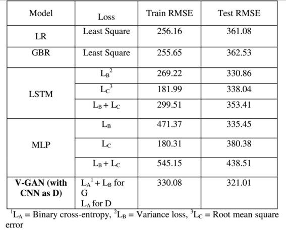
As shown in Table 4, the MLP model performed the best in training data; however, the V-GAN model outperformed all other models in correctly predicting the future expenditures in test data. Furthermore, we obtained better performance on test data when the variance loss function was used to train the MLP and LSTM models compared to other loss functions. Among the four ML models, the LSTM performed the best on test data, followed by the MLP, LR, and GBR models. The final LSTM model was trained with a 2-lag period, 128 epochs, 8 batch size, ReLU activation function, and Adam optimizer. The LSTM model contained one hidden layer with 16 neurons, one dropout layer with 20% dropout, and an output layer with 1 neuron. Similarly, the final MLP model was trained with a 2-lag period, 256 epochs, 4 batch size, ReLU activation function, and Adam optimizer. The MLP model contained one hidden layer with 8 neurons, one dropout layer with 20% dropout, and then an output layer with 1 neuron. The final GBR model contained 100 decision tree estimators with 12 as the maximum tree depth and 0.1 as the value of the learning rate. Moreover, as shown in Table 3 and 4, the V-GAN model outperformed other GAN-based prediction models and different ML models used in prior research for correctly predicting the medicine expenditures of patients on test data.
Discussion and Conclusion
The primary objective of this research was to evaluate the potential of generative adversarial networks (GANs) as a time-series model for predicting patients’ expenditures on medications. In this research, we experimented with different combinations of loss functions to train the generator and discriminator models in a GAN and proposed a novel variance-based GAN (V-GAN) architecture, which minimized the difference in variance between model and actual data explicitly. The generator model (G) in V-GAN was trained using the binary cross-entropy and the variance loss function, where the discriminator model (D) was trained using the binary cross-entropy loss function. This research systematically evaluated the use of different loss functions in GAN’s training for generating time-series dataset related to patients’ expenditures on a medication. Moreover, the proposed V-GAN model’s performance was also compared against a linear regression (LR), a gradient boosting regression (GBR), a multilayer perceptron (MLP), and a long short-term memory (LSTM) model for predicting the multivariate time-series dataset.
First, we found that the proposed V-GAN model outperformed all the other GAN-based models (developed with different loss functions) for predicting patients’ average expenditure on a weekly level. A likely reason for this result is that reducing the difference in variance between model and patients’ data during model training helped obtain a lower RMSE on test data. Next, we found that the V-GAN model outperformed LR, GBR, MLP, and LSTM models in this research on test data. Additionally, we obtained better performance from the MLP and LSTM models trained with the variance loss function compared to when these models were trained with the other loss functions. Therefore, we found a consistent behavior of the time-series prediction models, which implies that variance minimization for model and actual data during training helps generate better predictions. Furthermore, among LR, GBR, MLP, and LSTM models, the LSTM outperformed others. LSTM’s performance was followed by MLP, LR, and GBR. A likely reason for this result could be that the LSTM model can maintain memory states across sequences and produce superior performance for time-series predictions [34]. Overall, we conclude that GAN-based prediction models that focus on variance minimization can be developed in the healthcare domain and in other applications for generating time-series datasets. Additionally, developing LSTM based time-series models where loss function aims at reducing the variance difference between model and actual data might be helpful in general.
Second, we found that the Wasserstein distance (LW ) as a discriminator model’s loss function in the VW1-GAN model did not help the model generate correct predictions. This result is in contrast to prior results on image datasets, where the use of Wasserstein distance loss function resulted in better performance and stable training [23]. However, in this research, when LW was used as a discriminator model’s loss function, we experienced mode collapse and 0% real-like samples as a result reported by the discriminator. Mode collapse is a situation where the generator generates a limited diversity of samples, or even the same sample, regardless of the input [48]. This happens when the generator fails to model the distribution of the training data well enough. In the case of VW1-GAN, we found that after certain epochs, the model stopped learning, and it was generating the same samples again and again. In general, the generator is always trying to find the one output that seems most plausible to the discriminator. If the generator starts producing the same output (or a small set of outputs) over and over again, the discriminator’s best strategy is to learn always to reject that output. However, if the next generation of discriminator gets stuck in a local minimum and does not find the best strategy, then it is too easy for the next generator iteration to find the most plausible output for the current discriminator. Thus, in the VW1-GAN model, each iteration of the generator was over-optimized for a particular discriminator, and the discriminator never managed to find its way out of the trap. As a result, the generator rotated through a small set of output types and encountered mode-collapse. Also, using a combination of LA and LW loss functions for the discriminator did not help much in generating real-like samples, and we obtained only 11% real-like samples.
Next, we also experienced a minimal amount of overfitting from the V-GAN model (as shown in the train and test RMSE results reported in Table 3) compared to the other models. Additionally, when the variance loss function was present in the generator across all the GAN-based prediction models, the amount of overfitting reduced compared to when the variance loss function was absent. Moreover, for MLP and LSTM models, the variance loss function helped these models reduce the overfitting (as shown in the train and test RMSE results reported in Table 4) compared to the forecast error loss function. Therefore, the reduction in the difference in variance between model and actual data is in general useful for time-series forecasting models.
From the above results, we imply that the proposed V-GAN model can be utilized as a prediction model to generate/predict time-series datasets in the healthcare domain. The advantage of using V-GAN over existing models in this domain is that the GAN-based models generate future data that will have similar distribution as the actual patients’ data. Whereas, methods like regression, bagging, and boosting do not care about the underlying data distributions while predicting future outcomes. Moreover, it is clear from the experiment shown in this research that the V-GAN model has the potential to produce robust and accurate results compared to other popular time-series models such as LSTMs. That is because the V-GAN model minimizes the difference in variance between model and actual data by reducing the gap between generated values and the mean value of the distribution. Additionally, GAN is an unsupervised learning approach. Therefore, we do not need to worry about providing labels or the lag values (i.e., values on prior time-steps) in the V-GAN model, as we need to train other existing time-series prediction models.
A drawback of the proposed method is model training: GAN-based prediction models are harder to train compared to other neural network models like MLP and LSTM. Furthermore, the GAN models may fail to model a multimodal probability distribution of data and can encounter mode collapse. Additionally, GAN models may experience slow convergence due to the internal covariate shift [48]. The internal covariate shift occurs when there is a change in input distribution to the network [48]. Due to changes in the input distribution, hidden layers may try to learn to adapt to the new distribution, which slows down the training process. If the training process slows down, it takes a long time to converge to a global minimum. Batch normalization technique may be one solution to avoid this problem during GAN training [48]. Though there are certain challenges associated with GAN models, these methods have the potential to generate accurate predictions.
In this research, we predicted the patients’ expenditure on medication, and our results are likely to hold for other patient-related time-series variables. Therefore, we believe that the V-GAN framework could be used for other medications after some fine-tuning of the proposed structure of generator and discriminator models. Developing GAN-based prediction models may be beneficial, where data is limited, and accuracy is the prime objective. The proposed models may help pharmaceutical companies optimize the medications’ manufacturing process and other industries for better inventory management. Apart from the healthcare domain, the proposed method could be used to predict stock market data, weather prediction, earthquake prediction, and for several other applications. As part of our future research, it would be worthwhile to explore V-GAN and other GAN-based prediction models for predicting patients-related expenditures on other medications.
