Introduction to Machine Learning with Random Forest (Pharma/Genetics)
To pick up where we left off last blog post, we discussed the potential of predictive analytics in the genetics of cancer. I aim to achieve this by using the aforementioned Random Forest classification algorithm.This powerful supervised learning algorithm has been documented to a great extent in the field of Machine Learning and is starting to find its feet in genetics (Touw et al., 2012) (Chen and Ishwaran, 2012). The algorithm will exploit the real world clinical evidence by taking a measure of the term frequency that occurs within all the analyzed clinical documents and compare it to that of the untouched clinical reports to predict a class for the genetic variants.
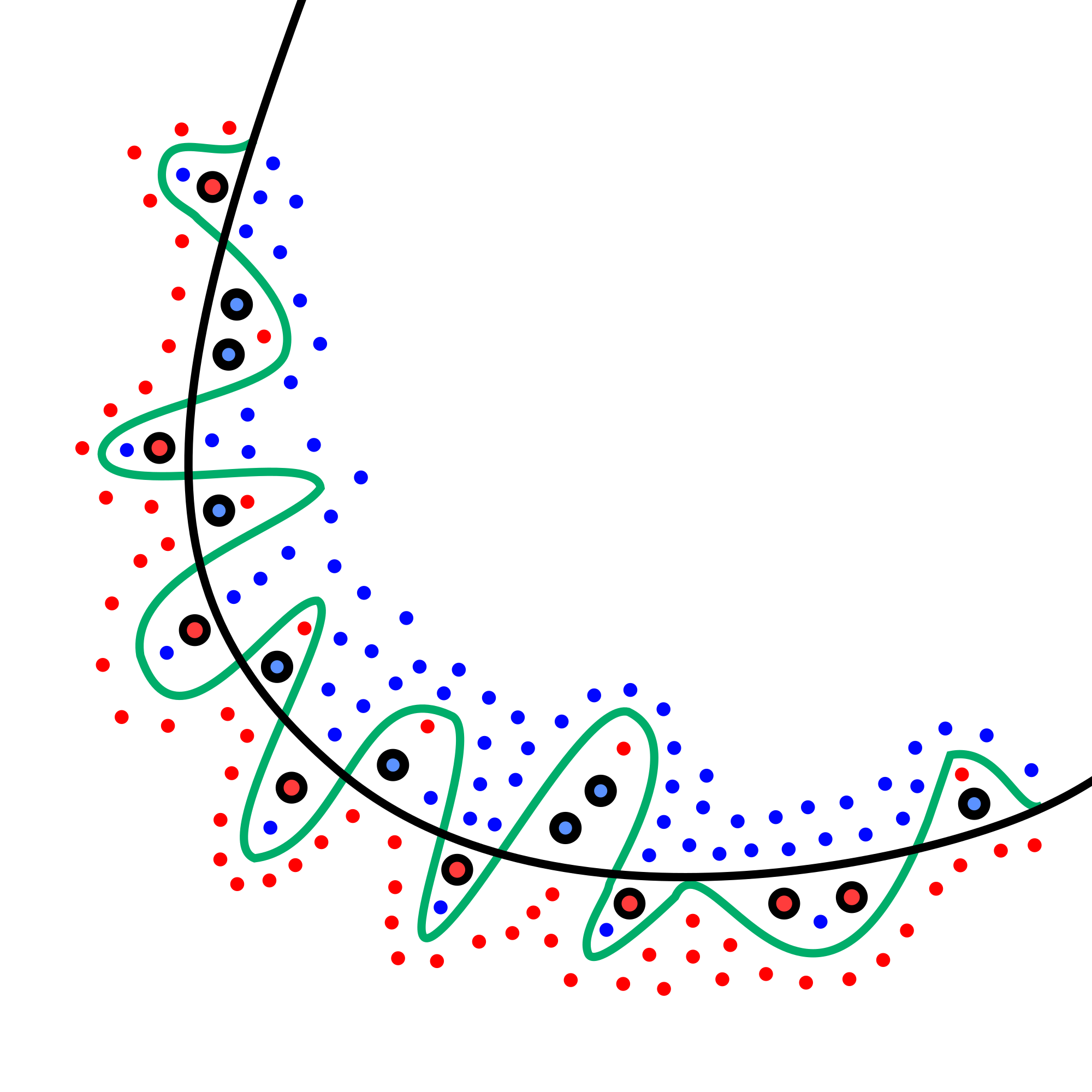
Before taking this conversation any further, it’s imperative that we discuss the nature of Random Forests to build a better understanding as to how we intend on interpreting this ever-complex dataset. Random Forests are built upon a more basal algorithm you may have heard of before - the Decision Tree (Ho, 1995). The problem with the Decision Tree is that as the complexity of the issue increases, the robustness of its future predictions decreases, particularly when dealing with as small a dataset as we have (Song et al., 2015). This is a one-way street to overfitting given the fact that we only have about 3,000 data samples to learn with, which would leave us with a less than optimal decision tree algorithm in reality (Rokach and Maimon, 2010). We can say this because the algorithm is now so specific to the training data at hand that it will be unable to think for itself should it come across any new variables in the test dataset and will therefore be unable to accommodate for said surprises (Hawkins, 2004). Thus, we look towards Random Forest.
Image from Wikimedia Commons
Random Forest works by averaging the results of many individual estimators which over-fit the data (Goel and Abhilasha, 2017). This makes it an ideal solution for this problem as the number of trees in the model can upscale alongside the complexity (Hastie, Tibshiriani and Friedman, 2009). This ensemble method minimizes the prediction variance which in turn improves the accuracy. The random forest classifier algorithm in sklearn uses a ‘perturb-and-combine’ technique which produces a unique set of trees or ‘classifiers’ which introduces the randomness into the equation that is classifier construction (Scikit-learn.org, 2018). An interesting twist in sklearn’s implementation of the algorithm is that it combines classifiers by averaging their probabilistic prediction rather than allowing each classifier to vote for a single class and then taking the mode of this output.
This may all sound well and good but how does this model bring me any closer to predicting the class of potentially oncogenic variants? To explore this further, we need to discuss text feature extraction. Of course, text analysis is a major utilization of machine learning - However, machine learning algorithms have always operated on numerical feature vectors with a fixed size rather than a sequence of symbols with variable lengths (Liang et al., 2017). To overcome this obstacle, we apply scikit-learn’s CountVectorizer to our data (Scikit-learn.org, 2018). This algorithm can convert our clinical text documents to meaningful, extractable numerical features by following these steps:
This conversion process can be referred to as Vectorization.
So, the CountVectorizer will tokenize and count the word occurrence of all our analyzed clinical documents (any word herein contains at least two characters). Each token is assigned an integer identification number which corresponds to a column in the resulting matrix. The entire body of clinical reports will each have a row in the same matrix, leaving us ready to implement the RandomForestClassifier algorithm (Scikit-learn.org, 2018).
It’s also essential for us to discuss the data at hand before diving any deeper into the Random Forest. Firstly, we have two datasets (namely the training and test dataset), each containing two distinct files (namely the genetic and text files). We merge the files via kdb+ to obtain 3,321 rows of genetic and text information for the training dataset and 5,668 rows for the test dataset. I must reiterate here that this problem is not as much a big data issue as it is a complex one. To calculate the accuracy of the classification algorithm, we must perform a train-test split (once again using kdb+) on the training set to delegate 70% of the data to be learnt upon by the algorithm and a further 30% to be validated upon by comparing actual results to those predicted by the algorithm.
Training Dataset with Class
Test Dataset without Class
Forest Classifiers always need two variables – One array with the independent variables and another with the dependent variables. The independent variable in our case will be the text from clinical documents and the dependent variable will be the assigned class which is based upon the variant’s respective text. Now our Random Forest algorithm can build its own association between specific counts of text feature and their correlating class.
Once the algorithm has learnt of this association, we can pass through it an entirely new validation dataset for which we provide only the text data and withhold the already-known class of the variant. We do this so we can get a feel for the accuracy of the algorithm before applying it to any actionable test dataset which allows us to gauge our confidence within the algorithm itself. The accuracy can be determined by comparing the class predicted by the algorithm for each individual variant to the actual class determined by skilled oncologists. This observation is represented by the confusion matrix below.
Finally, to increase confidence in the selection of our parameters within this model, we perform the hyperparameter optimization known as grid search with cross-validation (explained in more detail in X’s blog here) (Bergstra and Bengio, 2012). Furthermore, to get an absolute indicator as to how well our algorithm performed, we run cross-entropy loss. Cross-entropy loss, or log loss, measures the performance of a classification model whose output is a probability value between 0 and 1 (de Boer et al., 2005). Cross-entropy loss increases as the predicted probability diverges from the actual label i.e. a perfect model would have a log loss of 0. Data Scientists across the world compare one another’s algorithms using such a score – I suppose a little competition never hurt anybody!
Now that we have a strong accuracy score, we can move forward with classifying our test dataset for which we genuinely don’t know the class of the variant which is the ultimate end-goal for the task at hand. In our third and final week, we’ll investigate the all-important results and discuss the practicality of our prototype in the modern world of medicinal genetics in cancer.
About the Author
Conor Moran is a graduate of Genetics from University College Dublin and an aspiring data scientist. He is exploring the capabilities of machine learning within the life science disciplines where he is hoping to make a significant impact in years to come. Conor is currently working alongside RxDataScience to spearhead the efforts of changing the way we think about our genetic data from a clinical perspective.
References
Touw, W., Bayjanov, J., Overmars, L., Backus, L., Boekhorst, J., Wels, M. and van Hijum, S. (2012). Data mining in the Life Sciences with Random Forest: a walk in the park or lost in the jungle? Briefings in Bioinformatics, 14(3), pp.315-326.
Chen, X. and Ishwaran, H. (2012). Random forests for genomic data analysis. Genomics, 99(6), pp.323-329.
Ho, T. K. (1995). Random decision forests [Paywall]. In Document analysis and recognition, 1995, Proceedings of the third international conference, Montreal, Quebec, Canada (Vol. 1, pp. 278–282). New York City, NY: IEEE.
Hastie, T., Tibshiriani, R. and Friedman, J. (2009). The Elements of statistical learning. 2nd ed. New York: Springer, pp.587–588.
Rokach, L. and Maimon, O. (2010). Data mining with decision trees. New Jersey, London, Singapore: World Scientific, p.49.
Scikit-learn.org. (2018). 1.11. Ensemble methods — scikit-learn 0.19.1 documentation. [online] Available at: http://scikit-learn.org/stable/modules/ensemble.html#forest [Accessed 21 Mar. 2018].
Hawkins, D. (2004). The Problem of Overfitting. Journal of Chemical Information and Computer Sciences, 44(1), pp.1-12.
Goel, E. and Abhilasha, E. (2017). Random Forest: A Review. International Journal of Advanced Research in Computer Science and Software Engineering, 7(1), pp.251-257.
Liang, H., Sun, X., Sun, Y. and Gao, Y. (2017). Text feature extraction based on deep learning: a review. EURASIP Journal on Wireless Communications and Networking, 2017(1).
Scikit-learn.org. (2018). 4.2. Feature extraction — scikit-learn 0.19.1 documentation. [online] Available at: http://scikit-learn.org/stable/modules/feature_extraction.html#text-feature-extraction [Accessed 21 Mar. 2018].
de Boer, P., Kroese, D., Mannor, S. and Rubinstein, R. (2005). A Tutorial on the Cross-Entropy Method. Annals of Operations Research, 134(1), pp.19-67.
Bergstra, J., & Bengio, Y. (2012). Random search for hyper-parameter optimization. The Journal of Machine Learning Research, 13(1), 281-305
Song, Yan-Yan & Lu, Ying. (2015). Decision tree methods: applications for classification and prediction. Shanghai archives of psychiatry. 27. 130-5. 10.11919/j.issn.1002-0829.215044.